Chapter 5 — Practical Considerations, Limitations, and Further Resources
The previous chapters established why reduced-order representations are needed, how 0D cardiovascular models describe pressure–flow relationships, how the RCR Windkessel model represents downstream vascular load, and how these models can be dynamically coupled to three-dimensional CFD domains.
However, defining an RCR model and establishing the coupling equations does not by itself guarantee a physiologically meaningful simulation. The reliability of the resulting solution also depends on numerical setup, initialization, convergence behavior, parameter consistency, and careful interpretation of what a reduced-order model can—and cannot—represent.
This final chapter therefore focuses on the practical checks required when using 0D/RCR models, the most common sources of error, the interpretation of differences between reduced-order and three-dimensional results, and the principal limitations of lumped-parameter representations. It concludes with several resources and tools that can support further work in cardiovascular modeling.
How do we know when a coupled solution is reliable?
A transient cardiovascular simulation should not be evaluated only by whether the numerical solver reaches convergence within an individual time step. The solution must also evolve toward a repeatable physiological state over successive cardiac cycles.
When an RCR model contains compliance, its internal state depends on the pressure and volume history inherited from previous time steps. The initial state assigned at the beginning of a simulation is therefore generally not identical to the periodic state associated with the prescribed inflow and downstream parameters. Several cardiac cycles may be required before the influence of initialization becomes negligible.
A practical criterion is cycle-to-cycle periodicity. Flow and pressure waveforms from successive cardiac cycles should increasingly overlap, and quantities such as mean flow, systolic pressure, diastolic pressure, or cycle-averaged pressure should change only negligibly between consecutive cycles [1].
Conceptually,
once a periodic solution has been reached, where is the cardiac-cycle period [1].
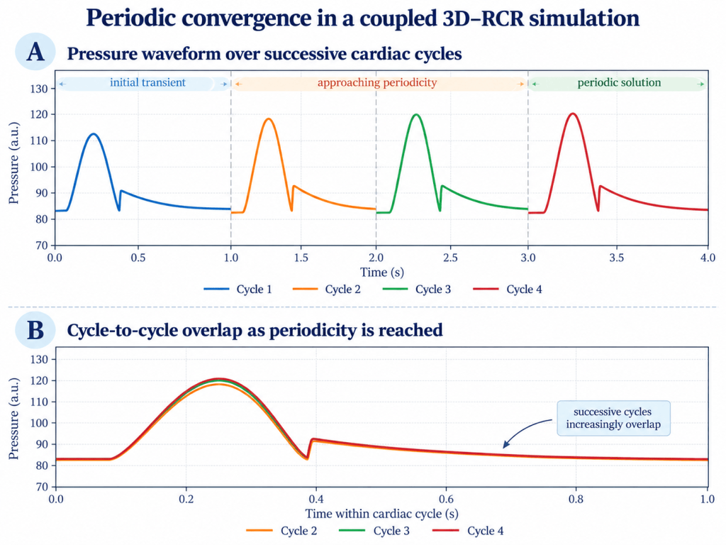
Figure 5.1. Periodic convergence in a coupled 3D–RCR simulation. (A) Pressure waveforms over successive cardiac cycles illustrate the decay of the initial transient and the progressive approach toward a periodic state. (B) When individual cycles are overlaid, successive pressure waveforms increasingly coincide, providing a practical criterion for assessing cycle-to-cycle convergence. A reliable periodic solution is reached when pressure and flow waveforms change negligibly between consecutive cardiac cycles.
The required number of cycles is not universal. It depends on the initial conditions, RCR time constants, imposed waveform, numerical scheme, and the overall cardiovascular model. Systems with relatively long characteristic time constants may retain the influence of their initial state for several cycles and therefore require longer transient simulations before periodic behavior is established [1].
Numerical convergence should also be accompanied by basic physical checks. For an incompressible rigid-wall 3D domain, inlet and outlet flow rates should satisfy conservation of mass within numerical tolerance,
and the resulting pressures and branch flows should remain within ranges consistent with the intended physiological condition.
Finally, the waveforms themselves should be inspected rather than relying exclusively on scalar convergence metrics. Unexpected oscillations, non-physiological pressure levels, discontinuities between time steps, or persistent cycle-to-cycle drift may indicate problems with initialization, boundary-condition implementation, parameter selection, or numerical resolution.
A reliable coupled solution therefore requires three complementary forms of assessment: numerical convergence within each time step, periodic convergence across cardiac cycles, and physiological plausibility of the resulting pressure and flow behavior [1,2].
Common pitfalls in 0D/RCR and 3D–RCR simulations
Even when the governing equations and coupling strategy are implemented correctly, relatively simple setup inconsistencies can produce pressure and flow responses that appear numerically stable but are physiologically incorrect. Several practical details therefore require careful attention.
One of the most common sources of error is unit inconsistency. Resistance, compliance, pressure, and flow may be reported in different unit systems across clinical measurements, 0D models, and CFD solvers. For example, converting between mmHg and Pa or between mL/s and m³/s changes the numerical magnitude of RCR parameters substantially. A parameter set that is physically reasonable in one unit system can become meaningless if transferred directly into another without consistent conversion.
The sign convention for outlet flow must also be defined explicitly. Depending on the CFD solver and surface-normal orientation, flow leaving the vascular domain may be reported as positive or negative. The RCR implementation must use a convention consistent with its governing equations; otherwise, the calculated pressure response may evolve in the wrong direction.
Another important consideration is the reference or distal pressure (). Resistance is fundamentally associated with a pressure difference rather than an absolute pressure. Using an inconsistent reference pressure when estimating RCR parameters and when applying them in the coupled simulation can therefore shift the resulting pressure waveform or alter the effective downstream load [6].
RCR parameters themselves should not be treated as arbitrary tuning constants. Values that reproduce a desired mean flow may still generate unrealistic systolic or diastolic pressures if the resistance partition or compliance is inappropriate. Mean pressure, pulse pressure, flow distribution, and waveform shape should therefore be considered together when evaluating a parameter set [5,6].
The physical time step also deserves attention. Because the RCR state evolves together with the transient CFD solution, an excessively large time step may fail to resolve rapid changes in flow or pressure and may introduce numerical errors into the coupling. Time-step sensitivity should therefore be assessed when the temporal resolution of the solution is uncertain [2].
Finally, results should not be interpreted before the initial transient has sufficiently decayed. As illustrated in Figure 5.1, a simulation may converge numerically within every time step while still exhibiting meaningful differences between successive cardiac cycles. Evaluating pressures or branch flows too early can therefore lead to conclusions that depend more on initialization than on the intended periodic cardiovascular state [1].
Many apparent problems in 3D–RCR simulations are therefore not caused by the RCR equations themselves, but by inconsistencies in units, conventions, reference states, parameter selection, temporal resolution, or convergence assessment. Checking these elements systematically is often more informative than attempting to correct unexpected results by modifying the downstream parameters alone.
How should differences between reduced-order and 3D models be interpreted?
Reduced-order and three-dimensional cardiovascular models describe the same circulation at different levels of spatial detail. Agreement between them should therefore be evaluated using quantities that both modeling approaches are capable of representing, rather than by expecting every aspect of the solutions to be identical [3,4].
A 0D model describes each vascular component through lumped pressure–flow relationships. It can reproduce quantities such as flow rate, mean or nodal pressure, resistance, compliance, and their evolution over time, but it does not resolve the spatial velocity or pressure field within a vessel. A 3D CFD model, in contrast, resolves local flow structures and spatial pressure variations throughout the vascular geometry [3,4].
For this reason, comparisons between the two approaches are most meaningful when they are based on consistent global or section-averaged quantities. Volumetric flow rate through the same vascular section, pressure averaged over an equivalent cross-section, mean branch flow fractions, or cycle-averaged hemodynamic quantities are generally more appropriate comparison metrics than local point values [3].
Even when inlet and downstream conditions are matched, small differences may remain. A three-dimensional geometry introduces viscous losses, curvature effects, branch interactions, secondary flow, and other local phenomena that are represented only in an aggregated manner—or may not be represented at all—in a lumped model. The effective hydraulic behavior of a realistic 3D vascular segment may therefore differ slightly from the idealized resistance or inertance assigned to its reduced-order counterpart [3,4].
Pressure comparisons require particular care. A 0D pressure usually represents a nodal or lumped pressure state, whereas pressure in a 3D domain varies spatially. Comparing a 0D value with pressure at an arbitrary CFD point can therefore create an apparent discrepancy that reflects the definition of the quantities rather than a true disagreement between the models. Whenever possible, the comparison location and pressure-averaging method should be defined consistently.
The same principle applies to phenomena that exist only in the higher-dimensional representation. Quantities such as local velocity profiles, recirculation zones, secondary flow structures, wall shear stress, or detailed spatial pressure gradients do not have direct 0D equivalents and should not be used as measures of reduced-order model agreement [3].
The objective of reduced-order validation is therefore not to reproduce every feature of a 3D solution. Instead, the key question is whether the reduced-order model captures the hemodynamic quantities it is designed to represent with sufficient accuracy for the intended application.
When interpreted in this way, differences between 0D and 3D models are not necessarily evidence that one model is incorrect. They may instead reflect the different spatial resolutions, assumptions, and physical information retained by each representation.
Capabilities, limitations, and from theory to practice
The strength of 0D/RCR modeling lies in its ability to reproduce important cardiovascular pressure–flow behavior using only a small number of state variables and parameters. When appropriately parameterized, an RCR model can represent downstream vascular resistance, arterial storage, pressure decay, and the dynamic load experienced by a coupled 3D vascular domain.
This makes lumped-parameter models particularly valuable when the quantities of interest are system-level hemodynamic variables. Mean and pulsatile pressure, volumetric flow rate, branch flow distribution, global vascular resistance, arterial compliance, and the interaction between a resolved vascular region and the surrounding circulation can often be investigated efficiently without explicitly reconstructing the entire cardiovascular system.
Their computational efficiency is another important advantage. Reduced-order models can be evaluated rapidly, making them useful for parameter studies, sensitivity analyses, preliminary boundary-condition estimation, and repeated testing of different physiological scenarios before substantially more expensive three-dimensional simulations are performed [3,4].
However, this efficiency is achieved by removing spatial information. As discussed above, a lumped model represents the overall pressure–flow behavior of the system rather than the detailed local hemodynamics within the vascular geometry. When spatially resolved flow phenomena are central to the research question, a higher-dimensional model is therefore required [3,4].
The same distinction applies to wave behavior. An RCR model can reproduce important features of the overall pulsatile pressure–flow response and downstream vascular load, but it does not explicitly resolve the spatial propagation of pressure and flow waves through a distributed arterial network. Detailed wave travel, reflection sites, and interactions associated with vessel length, branching, and spatially varying wall properties are more naturally represented by distributed models such as 1D vascular networks [4,5].
Standard RCR models also rely on simplifying assumptions. Resistance and compliance are typically represented as lumped and time-invariant parameters, whereas the physiological circulation may exhibit nonlinear vessel mechanics, active regulation of vascular tone, changing peripheral resistance, and other adaptive responses. Whether these effects need to be included depends on the physiological question being investigated and the level of fidelity required [4,5].
The appropriate modeling strategy should therefore be selected according to the question being asked. A reduced-order model is not intended to replace 3D CFD when detailed local hemodynamics are required, just as a full 3D model is not always necessary when the primary interest is global pressure–flow behavior. In many applications, the greatest value comes from combining different levels of representation so that each model contributes the information it is best suited to resolve.
Key idea: Reduced-order models are most useful when their simplicity is treated as a deliberate modeling choice rather than as a substitute for spatially resolved physics. The appropriate level of model complexity is the one that captures the information required to answer the physiological or engineering question of interest.
From theory to practice: the 0D-RCR Tool
The concepts introduced throughout this series also form the theoretical basis of the 0D-RCR Tool developed as part of this work. The software provides a practical environment for constructing reduced-order cardiovascular models, evaluating pressure–flow behavior, and determining outlet-specific RCR parameters that can subsequently be incorporated into three-dimensional cardiovascular CFD simulations.
The purpose of the tool is to provide a direct bridge between the theoretical principles discussed in these chapters and their practical application. Users can move from defining physiological targets and reduced-order vascular representations to evaluating the resulting hemodynamic response and generating RCR parameter sets for use as downstream boundary conditions in CFD workflows.
The objective of this series has therefore not been to identify a single “best” cardiovascular model, but to show how 0D representations, RCR Windkessel models, and 3D CFD can be understood as complementary components of a multiscale cardiovascular modeling framework. Used carefully, these approaches provide a practical bridge between physiological information, reduced-order analysis, and detailed computational hemodynamics.
References
[1] Pfaller MR, Pham J, Wilson NM, Parker DW, Marsden AL. On the periodicity of cardiovascular fluid dynamics simulations. Annals of Biomedical Engineering. 2021;49(12):3574–3592. doi: 10.1007/s10439-021-02796-x.
[2] Esmaily Moghadam M, Vignon-Clementel IE, Figliola R, Marsden AL, et al. A modular numerical method for implicit 0D/3D coupling in cardiovascular finite element simulations. Journal of Computational Physics. 2013;244:63–79. doi: 10.1016/j.jcp.2012.07.035.
[3] Pfaller MR, Pham J, Verma A, Pegolotti L, Wilson NM, Parker DW, Yang W, Marsden AL. Automated generation of 0D and 1D reduced-order models of patient-specific blood flow. International Journal for Numerical Methods in Biomedical Engineering. 2022;38(10):e3639. doi: 10.1002/cnm.3639.
[4] Shi Y, Lawford P, Hose R. Review of Zero-D and 1-D Models of Blood Flow in the Cardiovascular System. BioMedical Engineering OnLine. 2011;10:33. doi: 10.1186/1475-925X-10-33.
[5] Westerhof N, Lankhaar JW, Westerhof BE. The arterial Windkessel. Medical & Biological Engineering & Computing. 2009;47(2):131–141. doi: 10.1007/s11517-008-0359-2.
[6] Vignon-Clementel IE, Figueroa CA, Jansen KE, Taylor CA. Outflow boundary conditions for three-dimensional finite element modeling of blood flow and pressure in arteries. Computer Methods in Applied Mechanics and Engineering. 2006;195(29–32):3776–3796. doi: 10.1016/j.cma.2005.04.014.
