0D-RCR Chapter 4

Chapter 4 — Coupling 0D/RCR Models with 3D CFD

The previous chapter introduced the RCR Windkessel model as a compact representation of the hemodynamic load imposed by the unresolved downstream circulation. Once an appropriate set of $R_p$ , $R_d$ , and $C$ parameters has been defined, the next step is to connect this reduced-order representation to a three-dimensional vascular model.

Coupling an RCR model to a 3D CFD domain allows the outlet boundary condition to evolve dynamically throughout the cardiac cycle. Rather than prescribing the complete outlet pressure response in advance, the downstream pressure is determined from the flow produced by the CFD solution and the state of the RCR model.

The three-element Windkessel (RCR) model is a zero-dimensional lumped-parameter representation of the downstream circulation. Coupling this model to the outlet of a 3D CFD domain therefore represents a specific instance of 3D–0D cardiovascular coupling. Throughout this chapter, this configuration is referred to as 3D–RCR coupling [1,2].

The central idea is the continuous exchange of two hemodynamic quantities at the interface between the models: flow and pressure. The 3D domain provides the flow entering the downstream circulation, while the RCR model determines the corresponding pressure response. Repeating this exchange over successive time steps creates a feedback mechanism through which the resolved vascular domain and the unresolved downstream circulation influence one another.

From a static outlet condition to dynamic 3D–RCR coupling

A conventional CFD outlet boundary condition may prescribe a constant pressure or a predefined pressure waveform. In either case, the pressure condition is specified independently of the instantaneous flow generated by the three-dimensional solution. Such approaches can be useful in simplified simulations, but they do not allow the downstream vascular load to adapt dynamically to changes in the calculated flow [1,4,5].

A coupled RCR boundary condition behaves differently. The outlet pressure is not fully prescribed beforehand. Instead, the instantaneous flow rate leaving the 3D domain, $Q(t)$ , is supplied to the corresponding RCR model, which determines the pressure response according to its resistance, compliance, and current internal state [1,2].

Conceptually,

Q(t) \quad \longrightarrow \quad \text{RCR model} \quad \longrightarrow \quad P(t)

Because the RCR model contains a compliant element, its response also depends on the hemodynamic history of the system. The pressure at a given time therefore reflects not only the current flow rate but also the volume previously stored within the compliant compartment.

At each physical time step, the resulting RCR pressure is applied to the corresponding outlet of the 3D domain. This updated pressure influences the subsequent CFD solution and therefore alters the flow entering the RCR model at the following time step. The repeated exchange establishes a continuous pressure–flow feedback loop throughout the transient simulation.

The outlet boundary condition is consequently both flow-dependent and time-dependent. The 3D CFD model resolves the local velocity and pressure fields within the explicitly reconstructed vascular geometry, while the RCR model supplies the dynamic downstream load associated with the circulation that lies beyond it.

This interaction is the essential distinction between prescribing an outlet pressure and dynamically coupling the vascular domain to an RCR Windkessel model.

How are flow and pressure exchanged between the 3D and RCR models?

The interface between the 3D CFD domain and an RCR model is defined by two primary quantities: the flow rate leaving the vascular outlet and the pressure imposed by the downstream circulation. These variables are exchanged repeatedly as the transient solution advances in time.

At a given physical time step, the CFD solver first provides the instantaneous flow rate through an outlet,

Q_i(t) = \int_{A_i} u \cdot n \, dA

where $A_i$ is the outlet surface, $\mathbf{u}$ is the local velocity vector, and $\mathbf{n}$ is the outward unit normal. The subscript $i$ identifies the individual vascular outlet [2].

This flow rate becomes the input to the corresponding RCR model. Using the prescribed $R_{p,i}$ , $R_{d,i}$ , and $C_i$ parameters together with the internal state carried from the preceding time step, the RCR equations are advanced to determine the updated pressure response.

Conceptually, the exchange can be represented as

Q_i(t) \quad \longrightarrow \quad \mathrm{RCR}_i \quad \longrightarrow \quad P_i(t)

The calculated $P_i(t)$ is then applied as the pressure boundary condition at the same 3D outlet. The CFD solution subsequently responds to this updated downstream pressure, producing a new velocity field and therefore a new outlet flow rate as the simulation advances [2,5].

The process is repeated throughout the cardiac cycle:

\text{3D flow} \quad \rightarrow \quad \text{RCR update} \quad \rightarrow \quad \text{outlet pressure} \quad \rightarrow \quad \text{3D flow response}

The compliant component of the RCR model is particularly important in this exchange because it introduces memory into the boundary condition. The pressure at the current time step is not determined solely by the current outlet flow; it also depends on the state of the compliant compartment inherited from previous time steps. The downstream model therefore retains information about the recent hemodynamic history of the circulation.

In numerical terms, the exact sequence used to update flow, internal RCR state, and outlet pressure may vary with the coupling algorithm and CFD implementation. However, the underlying physical principle remains the same: the 3D solution supplies flow to the downstream model, and the downstream model returns a pressure response that influences the evolving 3D solution [2].

This repeated exchange transforms the RCR model from a prescribed boundary specification into an active component of the transient cardiovascular simulation.

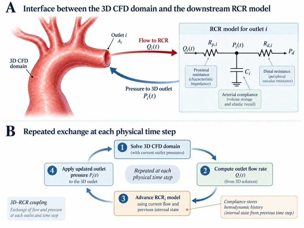
Figure 4.1. Schematic illustration of dynamic 3D–RCR coupling at a vascular outlet. (A) The outlet flow rate computed by the 3D CFD domain is supplied to the corresponding RCR model, which returns a time-dependent pressure to the same outlet. (B) This exchange is repeated at each physical time step, creating a dynamic pressure–flow feedback loop between the resolved vascular domain and the downstream circulation. The compliant element carries the hemodynamic state from one time step to the next.

How does downstream loading influence 3D hemodynamics?

Dynamic RCR coupling is important because the downstream vascular load can directly influence the hemodynamics resolved within the three-dimensional domain.

A greater downstream resistance generally requires a larger pressure difference to sustain a given flow, whereas a lower resistance allows blood to leave the modeled domain more readily. Arterial compliance also modifies the transient response by buffering pressure changes and influencing how rapidly pressure evolves throughout the cardiac cycle [1,4,5].

Consequently, the selected RCR parameters can affect not only the outlet pressure waveform but also the flow rate, pressure field, and pulsatile behavior within the resolved vascular geometry. In models containing several outlets, differences in downstream loading can additionally alter how the total flow is distributed among individual branches.

The downstream circulation should therefore be regarded as an active part of the modeled hemodynamic system rather than as a passive numerical termination of the 3D geometry. This becomes particularly important when different vascular territories are represented by separate outlet-specific RCR models.

Coupling multiple vascular outlets

Most cardiovascular CFD models contain more than one outlet. An aortic model, for example, may include branches supplying the head and upper extremities, visceral organs, kidneys, and lower-body circulation. Because each outlet connects to a different downstream vascular territory, the same boundary condition does not necessarily represent all branches appropriately.

In a multi-outlet 3D–RCR model, each outlet $i$ can therefore be connected to its own RCR representation [1,4,5],

\text{RCR}_i = (R_{p,i},\ R_{d,i},\ C_i)

with the corresponding flow and pressure exchange occurring independently at each interface.

At every physical time step, the 3D solver determines the flow rate leaving each outlet,

Q_1(t),\ Q_2(t),\ \dots,\ Q_N(t)

and each value is supplied to its associated RCR model. The downstream models then return the corresponding outlet pressures,

P_1(t),\ P_2(t),\ \dots,\ P_N(t)

which are applied simultaneously to the respective boundaries of the three-dimensional domain.

Importantly, the resulting branch flows are not determined by the RCR models in isolation. They emerge from the combined effects of the inlet condition, vascular geometry, local three-dimensional flow resistance, and outlet-specific downstream loads. A change in the RCR parameters at one outlet can therefore alter not only the flow through that branch but also the distribution of flow among the remaining outlets [1,4].

For a vascular domain with $N$ outlets, conservation of mass requires the total outflow to remain consistent with the inflow:

Q_{\mathrm{in}}(t) \approx \sum_{i=1}^{N} Q_i(t)

for an incompressible rigid-wall vascular domain.

This coupled behavior is particularly important when different branches supply vascular territories with substantially different physiological demands. Outlet-specific RCR models allow these differences in downstream loading to be represented without explicitly reconstructing the entire distal arterial network.

The multi-outlet formulation therefore extends the same 3D–RCR coupling principle introduced for a single outlet: each branch communicates dynamically with its own downstream representation, while all outlets remain interconnected through the shared three-dimensional flow field.

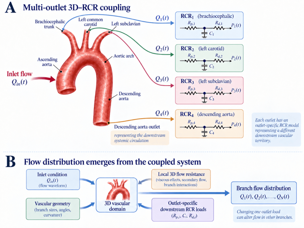
Figure 4.2. Multi-outlet 3D–RCR coupling and the determinants of branch flow distribution. (A) Each vascular outlet is coupled to an outlet-specific RCR model representing the downstream load of a distinct vascular territory; the truncated descending aorta represents the remaining systemic circulation. (B) The resulting branch flow distribution emerges from the combined effects of the inlet condition, vascular geometry, local 3D flow resistance, and outlet-specific RCR loads. Consequently, modifying the downstream load at one outlet can influence flow through the other branches.

From coupling mechanics to practical implementation

The numerical implementation of 3D–RCR coupling can vary between CFD solvers. The RCR equations may be incorporated through built-in boundary-condition frameworks, custom coupling routines, or user-defined functions that update the outlet pressure as the transient solution advances. Regardless of the implementation, the underlying principle remains unchanged: outlet flow is supplied to the downstream model, the RCR state is advanced in time, and the resulting pressure is returned to the corresponding 3D boundary [2].

For multi-outlet vascular models, this exchange occurs simultaneously across all coupled boundaries, allowing the three-dimensional flow field and the outlet-specific downstream loads to evolve as part of a single hemodynamic system. The resulting solution therefore reflects both the local behavior resolved within the vascular geometry and the global influence of the circulation represented beyond its outlets.

Establishing the coupling equations, however, is only one part of building a reliable cardiovascular simulation. The choice of time step, initialization of the RCR state, attainment of periodic behavior, consistency of units and sign conventions, and interpretation of differences between reduced-order and 3D results can all influence the quality of the final solution. These practical considerations, together with the principal capabilities and limitations of 0D/RCR modeling, are discussed in Chapter 5.

References

[1] Vignon-Clementel IE, Figueroa CA, Jansen KE, Taylor CA. Outflow boundary conditions for three-dimensional finite element modeling of blood flow and pressure in arteries. Computer Methods in Applied Mechanics and Engineering. 2006;195(29–32):3776–3796. doi: 10.1016/j.cma.2005.04.014.

[2] Esmaily Moghadam M, Vignon-Clementel IE, Figliola R, Marsden AL, for the MOCHA Investigators. A modular numerical method for implicit 0D/3D coupling in cardiovascular finite element simulations. Journal of Computational Physics. 2013;244:63–79. doi: 10.1016/j.jcp.2012.07.035.

[3] Kim HJ, Vignon-Clementel IE, Figueroa CA, LaDisa JF, Jansen KE, Feinstein JA, Taylor CA. On coupling a lumped parameter heart model and a three-dimensional finite element aorta model. Annals of Biomedical Engineering. 2009;37(11):2153–2169. doi: 10.1007/s10439-009-9760-8.

[4] Pirola S, Cheng Z, Jarral OA, O’Regan DP, Pepper JR, Athanasiou T, Xu XY. On the choice of outlet boundary conditions for patient-specific analysis of aortic flow using computational fluid dynamics. Journal of Biomechanics. 2017;60:15–21. doi: 10.1016/j.jbiomech.2017.06.005.

[5] Madhavan S, Cherry Kemmerling EM. The effect of inlet and outlet boundary conditions in image-based CFD modeling of aortic flow. BioMedical Engineering OnLine. 2018;17:66. doi: 10.1186/s12938-018-0497-1.

Chapter 3 ← Previous

↑ Back to Contents

Next → Chapter 5