0D-RCR Chapter 2

Chapter 2 — Fundamentals of 0D Cardiovascular Modeling

**What does “zero-dimensional” mean?**

In a three-dimensional cardiovascular model, pressure and velocity vary throughout both space and time. A CFD simulation may therefore describe a velocity field

\mathbf{u}=\mathbf{u}(x,y,z,t)

and a pressure field

P=P(x,y,z,t)

A zero-dimensional (0D) model takes a fundamentally different approach. Instead of resolving the spatial distribution of pressure and velocity within the vascular domain, the cardiovascular system is represented by a set of interconnected lumped elements. Each element is described using a limited number of variables, such as pressure, volumetric flow rate, and blood volume.

The primary hemodynamic variables are therefore expressed as functions of time rather than explicit spatial coordinates:

P=P(t)

Q=Q(t)

This is the meaning of zero-dimensional. It does not mean that vascular geometry has no influence on the model. Rather, the spatial characteristics of a vessel or vascular region are condensed into lumped parameters that represent its dominant hemodynamic behavior.

For example, vessel dimensions, wall properties, and blood viscosity may ultimately influence parameters describing resistance, compliance, or inertial effects, without requiring the detailed three-dimensional flow field to be resolved.

As a result, a vascular system containing many anatomical components can be represented by a relatively small system of algebraic and ordinary differential equations. This substantial reduction in model complexity makes 0D simulations computationally inexpensive while preserving the pressure–flow relationships that are most important for global cardiovascular hemodynamics [1, 6].

From a blood vessel to a lumped element

Consider a short segment of an artery.

In reality, blood flowing through this segment is governed by several interacting physical effects. Viscous friction causes a pressure loss along the vessel. The arterial wall expands and recoils as pressure changes, allowing blood volume to be temporarily stored. The blood itself has mass, so accelerating or decelerating the flow requires an additional pressure difference.

A three-dimensional fluid or fluid–structure interaction model represents these effects by resolving the governing equations throughout the vascular domain.

A 0D model takes a different approach.

Instead of resolving the detailed spatial flow field, the dominant behavior of the vessel segment is represented using a small number of lumped elements [1, 2]. The most commonly used elements are:

Resistance (R), representing viscous opposition to blood flow.
Compliance (C), representing the ability of the vessel or vascular bed to store blood volume as pressure changes.
Inertance (L), representing the inertia of the moving blood and its resistance to rapid changes in flow.

The original vascular segment can therefore be replaced conceptually by an equivalent lumped representation, as illustrated in Figure 2.1.

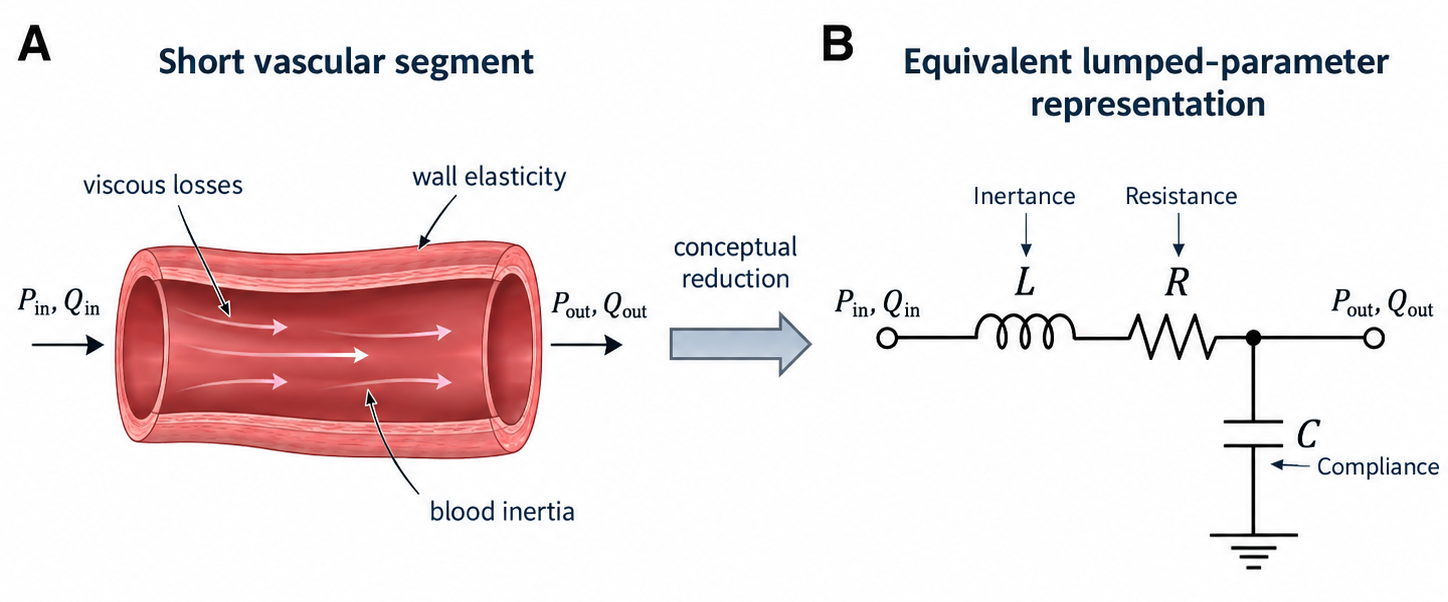
[ \text{vascular segment} \quad \longrightarrow \quad R;C;L ]

Figure 2.1. Conceptual reduction of a short vascular segment into an equivalent lumped-parameter representation. (A) A short vascular segment illustrating the dominant physical effects governing blood flow, including viscous losses, wall elasticity, and blood inertia, together with inlet and outlet variables ( $P_{\mathrm{in}}, Q_{\mathrm{in}}$ ) and ( $P_{\mathrm{out}}, Q_{\mathrm{out}}$ ). (B) A possible lumped-parameter representation, in which these effects are represented by inertance (L), resistance (R), and compliance (C).

The objective is not to reproduce every local feature of the velocity field. Instead, the model preserves the input–output hemodynamic behavior of the vascular region: how flow entering the segment is related to pressure, how much blood volume can be temporarily stored, and how the system responds to changes over time.

This distinction is fundamental.

A 0D element should not be interpreted as a miniature anatomical vessel. It is a mathematical representation of the dominant physical behavior of the anatomical region that it replaces.

For example, two vascular regions with different geometries may still exhibit similar lumped hemodynamic behavior if their effective resistance and compliance are comparable. Conversely, relatively small changes in vessel caliber or wall stiffness may substantially alter the corresponding lumped parameters even though the network topology remains unchanged.

Once individual vascular regions are represented in this way, they can be connected to form a larger network. Pressure is assigned to nodes, flow passes between those nodes, and conservation laws determine how the elements interact.

This is the basis of lumped-parameter cardiovascular modeling.

The next step is to understand why these hydraulic elements can be represented so naturally using an electrical-circuit analogy.

The electrical analogy

The mathematical structure of a 0D cardiovascular model closely resembles that of an electrical circuit. This analogy provides an intuitive and convenient framework for translating vascular behavior into interconnected lumped elements.

The fundamental correspondence is between pressure and voltage, and between volumetric flow rate and electrical current. A pressure difference drives blood through the circulation in much the same way that a voltage difference drives electrical current through a circuit.

The principal hydraulic–electrical analogies can be summarized as follows:

Cardiovascular quantity	Electrical analogue
Pressure ( $P$ )	Voltage ( $V$ )
Pressure difference ( $\Delta P$ )	Voltage difference ( $\Delta V$ )
Volumetric flow rate ( $Q$ )	Electrical current ( $I$ )
Hydraulic resistance ( $R$ )	Electrical resistance
Vascular compliance ( $C$ )	Capacitance
Blood inertance ( $L$ )	Inductance

This correspondence is more than a visual analogy. The governing relationships of the hydraulic elements have the same mathematical form as those of their electrical counterparts.

For a resistive element,

\Delta P = RQ

which corresponds directly to Ohm’s law,

\Delta V = RI

For a compliant element, the flow associated with volume storage is related to the rate of pressure change:

Q_C = C\frac{dP}{dt}

This is analogous to the current–voltage relationship of an electrical capacitor.

Similarly, the pressure difference required to accelerate or decelerate a fluid can be represented by an inertance:

\Delta P = L\frac{dQ}{dt}

which has the same mathematical form as the voltage–current relationship of an electrical inductor.

These equivalences explain the circuit representation introduced in Figure 2.1B. The resistor represents dissipative pressure losses, the capacitor represents temporary blood-volume storage associated with vascular compliance, and the inductor represents the inertia of the moving blood.

The analogy also extends naturally to vascular networks. At a junction, conservation of blood flow requires that the total flow entering the node balances the total flow leaving it, apart from any flow temporarily stored within a compliant compartment:

\frac{dV}{dt}

This is analogous to conservation of electrical current at a circuit node. Likewise, pressures assigned to nodes play a role analogous to electrical potentials, while differences between nodal pressures drive flow through the connecting elements.

As a result, a complex cardiovascular system can be represented as a network of pressure nodes connected by resistive, compliant, and inertial elements. The resulting circuit is not intended to imply that blood vessels behave literally as electrical components. Rather, the electrical representation provides a compact mathematical language for describing equivalent relationships between pressure, flow, storage, and inertia [1, 2].

With this analogy established, the physical meaning of each lumped element can now be examined individually, beginning with the simplest: hydraulic resistance.

Resistance: opposition to flow

Hydraulic resistance describes the opposition of the vascular system to blood flow. In a 0D model, it provides the simplest relationship between pressure difference and volumetric flow rate.

For a purely resistive element,

\Delta P = RQ

where ( $\Delta P$ ) is the pressure difference across the element, ( $Q$ ) is the volumetric flow rate, and ( $R$ ) is the hydraulic resistance.

Equivalently,

R=\frac{\Delta P}{Q}

This relationship is the hydraulic analogue of Ohm’s law. A larger resistance requires a larger pressure difference to maintain the same flow, whereas for a given pressure difference, an increase in resistance results in a decrease in flow.

The physical origin of vascular resistance is primarily viscous friction between the moving blood and the vessel wall, as well as internal viscous interactions within the fluid.

For steady, fully developed, laminar flow of a Newtonian fluid through a rigid cylindrical tube, the relationship can be expressed using the Hagen–Poiseuille equation:

R=\frac{8\mu \ell}{\pi r^4}

where ( $\mu$ ) is the dynamic viscosity of blood, ( $\ell$ ) is the vessel length, and ( $r$ ) is the vessel radius

This expression illustrates an important feature of vascular resistance: it is highly sensitive to vessel diameter. Because resistance varies inversely with the fourth power of radius,

R \propto \frac{1}{r^4}

even a relatively small change in vessel radius can produce a substantial change in resistance.

By comparison, resistance increases linearly with both vessel length and fluid viscosity:

R \propto \mu \ell

These relationships help explain why small arteries and arterioles play such an important role in controlling systemic vascular resistance. Although large arteries carry substantial blood flow, their relatively large diameters produce comparatively low hydraulic resistance.

In a 0D cardiovascular model, however, a resistance element does not necessarily represent a single cylindrical vessel. It may instead represent the effective resistance of an entire vascular region, such as a distal arterial tree or peripheral vascular bed. In such cases, the parameter ( $R$ ) summarizes the overall pressure loss associated with many unresolved vessels.

For vascular elements connected in series, the equivalent resistance is

R_1+R_2+\cdots+R_n

For elements connected in parallel,

\frac{1}{R_1} + \frac{1}{R_2} +\cdots+ \frac{1}{R_n}

These relationships are particularly useful when constructing lumped cardiovascular networks containing multiple vascular branches.

A purely resistive element, however, responds instantaneously to changes in flow. It cannot represent the ability of elastic arteries to temporarily store blood during systole and release it during diastole.

To describe that behavior, a second fundamental element is required: vascular compliance.

Compliance: storing blood volume

Blood vessels are not rigid conduits. Their walls deform in response to changes in pressure, allowing the vascular system to temporarily store and release blood volume throughout the cardiac cycle.

This behavior is represented in a 0D model by vascular compliance.

Compliance is defined as the change in blood volume associated with a change in pressure:

C=\frac{dV}{dP}

where $C$ is vascular compliance, $V$ is blood volume, and $P$ is pressure.

For a linear compliant element, this relationship may be approximated as

\Delta V=C,\Delta P

A highly compliant vascular region can therefore accommodate a relatively large change in blood volume with only a small increase in pressure. Conversely, a stiff vascular region has lower compliance and undergoes a smaller volume change for the same pressure variation.

Because changes in stored blood volume are associated with flow, the flow entering a compliant element can be written as

Q_C=\frac{dV}{dt}

Combining this expression with the definition of compliance gives

Q_C=C\frac{dP}{dt}

for a constant compliance.

This equation introduces an important feature that is absent from a purely resistive element: time dependence.

Resistance relates pressure and flow instantaneously,

\Delta P=RQ

whereas compliance allows part of the incoming flow to be temporarily stored as vascular volume. The pressure response therefore depends on how the system has evolved over time.

This behavior is central to arterial hemodynamics.

During systole, ventricular ejection delivers blood into the arterial system faster than it can immediately leave through the peripheral circulation. Part of this excess volume is temporarily accommodated by expansion of the compliant arteries.

During diastole, when ventricular ejection has ceased, elastic recoil of the arterial walls releases part of this stored volume and continues to drive blood toward the peripheral circulation.

This storage-and-release mechanism smooths the strongly pulsatile output of the heart and helps maintain pressure and forward flow between successive ventricular ejections.

In a lumped-parameter model, a compliance element therefore represents more than the deformability of a single vessel. Depending on the model scale, it may represent the combined volume-storage capacity of an entire vascular region.

Large elastic arteries, particularly the aorta and its major branches, make an important contribution to arterial compliance because their walls expand appreciably during systolic pressure elevation. Distal vascular regions may also contribute distributed compliance that can be lumped into an equivalent parameter when spatial details are not explicitly modeled.

Just as resistances can be combined into an equivalent resistance, multiple compliant regions can also be represented by an effective compliance when appropriate. For compliant elements exposed to the same pressure variation, such as idealized parallel capacitances,

C_1+C_2+\cdots+C_n

The value of compliance is therefore determined not only by vessel dimensions but also by the mechanical properties of the vascular wall. A reduction in wall distensibility, such as that associated with arterial stiffening, results in lower compliance and alters the relationship between pressure and stored blood volume.

Compliance also interacts directly with resistance. When a resistance and compliance are combined, they introduce a characteristic time scale into the system:

\tau=RC

where $\tau$ is the time constant.

This parameter describes how rapidly pressure changes within the compliant compartment. A larger value of $RC$ produces a slower pressure decay, whereas a smaller value produces a faster response.

The $RC$ time constant becomes particularly important in Windkessel models, where resistance and compliance together determine the diastolic pressure decay and the dynamic pressure–flow behavior of the downstream circulation.

Resistance and compliance are sufficient to describe much of the behavior required in many cardiovascular 0D models. However, neither accounts directly for the fact that blood has mass and therefore resists rapid acceleration and deceleration.

That effect is represented by the third fundamental lumped element: blood inertance.

Inertance: opposing changes in flow

Blood has mass, and therefore its flow cannot accelerate or decelerate instantaneously without a corresponding pressure force.

In a 0D model, this effect is represented by blood inertance.

For an inertial element, the pressure difference required to change the flow rate is expressed as

\Delta P=L\frac{dQ}{dt}

where $L$ is the inertance, $Q$ is the volumetric flow rate, and $dQ/dt$ represents the rate at which the flow changes with time.

This relationship is analogous to the voltage–current relationship of an electrical inductor.

Unlike resistance, which produces a pressure drop whenever flow is present, inertance becomes important when the flow is changing. A rapid increase or decrease in flow requires a larger pressure difference than a slowly varying flow.

For an idealized rigid cylindrical vessel containing an incompressible fluid, inertance can be approximated as

L=\frac{\rho \ell}{A}

where $\rho$ is the fluid density, $\ell$ is the vessel length, and $A$ is the cross-sectional area.

For a circular vessel,

A=\pi r^2,

and therefore

L=\frac{\rho \ell}{\pi r^2}

These relationships show that inertance increases with blood density and vessel length, while decreasing as the vessel cross-sectional area becomes larger.

The physical interpretation is straightforward: accelerating a larger mass of blood requires a greater pressure force. A long or narrow vascular segment contains a fluid column that is more difficult to accelerate than a short or wide segment.

Inertial effects are most relevant when flow changes rapidly, particularly in large proximal vessels and during the acceleration and deceleration phases of pulsatile flow. They may also become important in models involving valves, ventricular outflow, or other regions where rapid transient changes in flow occur.

In many peripheral vascular models, however, inertance is substantially less influential than resistance and compliance. For this reason, commonly used outlet models such as the three-element Windkessel model are often constructed using only resistive and compliant elements.

This does not mean that blood inertia is absent from the real circulation. Rather, its effect may be sufficiently small at the scale and location of interest that it can be neglected without substantially altering the desired hemodynamic response.

The decision to include $L$ should therefore depend on the purpose of the model and the temporal behavior that must be reproduced.

Together, resistance, compliance, and inertance describe three fundamental aspects of vascular behavior:

R \quad \longrightarrow \quad \text{viscous energy loss}

C \quad \longrightarrow \quad \text{blood-volume storage}

L \quad \longrightarrow \quad \text{opposition to flow acceleration}

By combining these elements, individual vascular regions can be assembled into larger 0D representations of the cardiovascular system.

The next step is therefore to move from individual lumped elements to the construction of a cardiovascular network.

Building a cardiovascular network

The main strength of 0D modeling appears when individual lumped elements are connected to represent larger portions of the cardiovascular system.

Pressure is assigned to network nodes, while flow passes through the resistive, compliant, and inertial elements connecting them. At an ideal junction with no volume storage, conservation of mass requires

\sum Q_{\text{in}} = \sum Q_{\text{out}}

If the network contains a compliant compartment capable of temporarily storing blood volume, the corresponding volume balance becomes

\sum Q_{\text{in}} – \sum Q_{\text{out}} = \frac{dV}{dt}

Thus, a positive flow imbalance increases the stored volume, whereas a negative imbalance decreases it.

By combining these conservation relationships with the constitutive equations of ( $R$ ), ( $C$ ), and ( $L$ ), a vascular network can be reduced to a system of algebraic and ordinary differential equations.

Such networks may represent anything from a single distal vascular bed to an entire closed-loop cardiovascular system.

Once this network perspective is established, the differences between 0D, 1D, and 3D cardiovascular models can be understood more clearly.

0D, 1D, and 3D models describe different levels of information

The distinction between 0D, 1D, and 3D cardiovascular models is not simply a progression from simple to advanced. Each formulation preserves a different level of spatial information and is therefore suited to different hemodynamic questions. The main differences between these model types are summarized schematically in Figure 2.2.

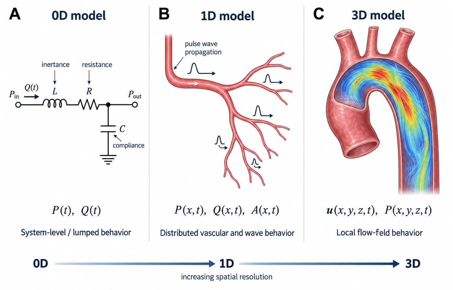
Figure 2.2. Comparison of 0D, 1D, and 3D cardiovascular models. (A) 0D models describe lumped, system-level pressure–flow behavior. (B) 1D models retain axial variation and capture distributed vascular and pulse-wave dynamics. (C) 3D models resolve local velocity and pressure fields within the vascular geometry. Moving from 0D to 3D increases spatial resolution and hemodynamic detail, together with computational complexity.

A 0D model describes the cardiovascular system using lumped pressure, flow, and volume variables. It is highly efficient and is especially useful for global hemodynamics, circulatory interactions, parameter estimation, and boundary-condition generation.

A 1D model retains variation along the vessel centerline. Pressure, flow rate, and cross-sectional area may therefore vary with axial position and time:

P=P(x,t), \qquad Q=Q(x,t), \qquad A=A(x,t)

This makes 1D models particularly useful for representing pulse-wave propagation and reflection throughout arterial networks.

A 3D model resolves the local velocity and pressure fields within the vascular geometry. It can therefore capture phenomena such as flow separation, recirculation, secondary flow structures, and local wall shear stress distributions.

Conceptually, the difference can be summarized as:

\text{0D} \quad \longrightarrow \quad \text{system-level / lumped hemodynamic behavior}

\text{1D} \quad\longrightarrow \quad \text{distributed vascular and wave behavior}

\text{3D} \quad\longrightarrow \quad \text{local flow-field behavior}

These approaches should therefore be regarded as complementary rather than competing models. A higher-dimensional model provides more spatial detail, but also requires greater computational effort and more detailed geometric and boundary-condition information.

This complementary perspective becomes particularly important when 0D models are coupled to 3D CFD domains, where they can provide a physiologically meaningful representation of the circulation that lies beyond the explicitly modeled anatomy [1, 3].

Why 0D models are especially useful for cardiovascular CFD

A three-dimensional CFD model resolves the local hemodynamics only within the explicitly modeled vascular geometry. The circulation beyond the outlets is therefore not directly included in the computational domain.

This creates an important boundary-condition problem.

If an outlet is assigned a fixed pressure, the downstream vascular response is greatly simplified. In reality, however, the distal circulation imposes a dynamic load that depends on both vascular resistance and the ability of compliant vessels to store and release blood.

A 0D model provides a practical way to represent this unresolved downstream circulation.

Instead of prescribing a constant outlet pressure, the pressure at the CFD boundary can be related dynamically to the flow leaving the domain:

Q_{\mathrm{out}} \quad \longrightarrow \quad \text{0D model} \quad \longrightarrow \quad P_{\mathrm{out}}

The 3D model therefore resolves the local velocity and pressure fields, while the 0D model represents the hemodynamic behavior of the vascular system that lies beyond the modeled anatomy.

This coupling allows the outlet pressure to evolve dynamically in response to the current flow, its previous state, and the properties assigned to the downstream circulation.

The result is a physiologically more meaningful interaction between the CFD domain and the rest of the cardiovascular system, without requiring the entire arterial tree to be modeled in three dimensions.

One of the most widely used 0D models for this purpose is the three-element Windkessel model, also known as the RCR model.

It combines a proximal resistance, a compliance, and a distal resistance to represent the dynamic pressure–flow behavior of the downstream arterial circulation [4 ,5].

References

[1] Shi Y, Lawford P, Hose R (2011) Review of zero-D and 1-D models of blood flow in the cardiovascular system. BioMedical Engineering OnLine 10:33. DOI: 10.1186/1475-925X-10-33.

[2] Westerhof N, Lankhaar JW, Westerhof BE (2009) The arterial Windkessel. Medical & Biological Engineering & Computing 47:131–141. DOI: 10.1007/s11517-008-0359-2.

[3] Formaggia L, Lamponi D, Quarteroni A (2003) One-dimensional models for blood flow in arteries. Journal of Engineering Mathematics 47:251–276. DOI: 10.1023/B.0000007980.01347.29.

[4] Vignon-Clementel IE, Figueroa CA, Jansen KE, Taylor CA (2006) Outflow boundary conditions for three-dimensional finite element modeling of blood flow and pressure in arteries. Computer Methods in Applied Mechanics and Engineering 195:3776–3796. DOI: 10.1016/j.cma.2005.04.014.

[5] Quarteroni A, Veneziani A (2003) Analysis of a geometrical multiscale model based on the coupling of ODEs and PDEs for blood flow simulations. Multiscale Modeling & Simulation 1:173–195. DOI: 10.1137/S1540345902408482.

[6] Pfaller MR, Pham J, Verma A, Pegolotti L, Wilson NM, Parker DW, Yang W, Marsden AL (2022) Automated generation of 0D and 1D reduced-order models of patient-specific blood flow. International Journal for Numerical Methods in Biomedical Engineering 38(10):e3639. DOI: 10.1002/cnm.3639.

Chapter 1 ← Previous

↑ Back to Contents

Next → Chapter 3